Tutorials#
The following docs page provides tutorials on how to use PySEP “in the wild” for research or teaching purposes. They are designed around using PySEP as a research tool for seismology or geophysical related problems.
Lab: Analyzing Seismic Data in Record Sections#
The following lab exercises were created by Aakash Gupta and Carl Tape as a part of the Applied Seismology (GEOS 626/426) course at University of Alaska Fairbanks. The Jupyter Notebook for this class assignment can be found on GitHub
Note
This lab has been reformatted with respect to the course notebook for optimized readability on ReadTheDocs, but the material is otherwise the same as what is presented in the course.
Instructions#
The goal is to create different seismic record section plots. A seismic record section is a series of seismograms that is plotted in some particular order. Typically, the x-axis is time, and then the seismograms are separated in the y-direction and ordered by source-station distance or source-station azimuth.
There are two main procedures of this lab:
fetching waveforms from the IRIS Data Management Center.
plotting record sections of seismograms.
The two main procedures are executed using the software package PySEP, which uses ObsPy. Check PySEP’s data gathering and record section plot pages for details on the two procedures.
The bandpass filter that is applied to the seismograms can have a dramatic effect on what is visible. The frequency limits of the bandpass is one of several important choices that are needed when plotting record sections. Check the IRIS webpage for the SEED format seismic channel naming.
We will not be removing instrument responses, as we did in lab_response. However, removing the instrument response can easily be achieved with the same tools. The two reasons we do not remove the responses are:
it takes a bit longer, computationally.
it can significantly distort the shape of the unfiltered waveforms, especially ones that are “odd,” which, here, we are interested in.
Table of Contents#
The notebook is organized into 7 event examples -
Yahtse glacier calving event
Mw 7.5 earthquake in southeastern Alaska
explosion in Fairbanks
very low frequency (VLF) event near Kantishna
landslide near Lituya Bay
Mw 8.6 Indian Ocean (offshore Sumatra) recorded in Alaska, plus triggered earthquakes
6.1. triggered earthquake (Andreanof)
6.2. triggered earthquake (Nenana crustal)
6.3. triggered earthquake (Iliamna intraslab)
your own example
Spend some time to understand the two key parts of each example - - waveform extraction - plotting a record section
Notebook Preamble#
NOTE: The notebook is designed such that data for a given example is downloaded only once and stored for subsequent use.
%matplotlib widget

import matplotlib.pyplot as plt
import matplotlib.image as img
import numpy as np
import os
import warnings

from copy import copy
from obspy.core import UTCDateTime
from pysep import Pysep
from pysep.recsec import plotw_rs
# script settings

warnings.filterwarnings("ignore")
plt.rcParams['figure.figsize'] = 9, 6
def fetch_and_plot(event, duration, download, plotting, bandpass):

    '''
    - downloads seismograms and plot them in a record section based on user inputs
    - also plots a source station map corresponding to the downloaded data
    - uses PySEP's data download and record section plotting utilities for the same
    - does not download data if the output data directory already exists
    '''

    '''
    :type event: dict
    :param event: event details
    :type duration: dict
    :param duration: time range for for data requested
    :type download: dict
    :param download: data download parameters
    :type plotting: dict
    :param plotting: record section plotting parameters
    :type bandpass: dict
    :param bandpass: bandpass filter parameters
    '''

    # download data
    data_dir  = f'{download["output_dir"]}/{download["overwrite_event_tag"]}'
    overwrite = f'{download["overwrite"]}'

    if (not os.path.isdir(data_dir)) or (overwrite == 'True'):
        print('\npreparing to download data ....')
        ps = Pysep(**event,**duration,**download)
        ps.run()
    else:
        print('\ndata directory already exists, no data will be downloaded')


    # plot source station map
    print('plotting source station map ....')
    plt.figure()
    source_station_map = img.imread(f'{data_dir}/station_map.png')
    plt.imshow(source_station_map)
    plt.show()

    # plot the record section using Pyseps's record section plotting tool
    print('\nplotting record section ....')
    plotw_rs(**plotting, **bandpass)
# setting pysep's data download defaults

# list of networks to retrieve data from
# providing an explicit list of networks is safer than using the wildcard (*)
networks            = ('AK,AT,AU,AV,BK,CI,CN,CU,GT,IC,II,IM,IU,MS,TA,TS,US,'
                       'XE,XM,XR,YM,YV,XF,XP,XZ')
# \networks            = '*'

download_defaults   = dict( networks                     = networks,
                            stations                     = '*',
                            locations                    = '*',
                            channels                     = 'BHZ',
                            maxdistance_km               = 200,
                            remove_clipped               = False,
                            remove_insufficient_length   = False,
                            fill_data_gaps               = 0,
                            remove_response              = False,
                            log_level                    = 'INFO',
                            plot_files                   = 'map',
                            output_dir                   = 'datawf',
                            sac_subdir                   = '',
                            overwrite_event_tag          = f'',
                            overwrite                    = False )
# setting pysep's record section plotting defaults

plotting_defaults   = dict( pysep_path                   = '',
                            sort_by                      = 'distance',
                            scale_by                     = 'normalize',
                            amplitude_scale_factor       = 1,
                            time_shift_s                 = None,
                            preprocess                   = 'st',
                            max_traces_per_rs            = None,
                            distance_units               = 'km',
                            tmarks                       = [0],
                            save                         = '',
                            log_level                    = 'CRITICAL' )
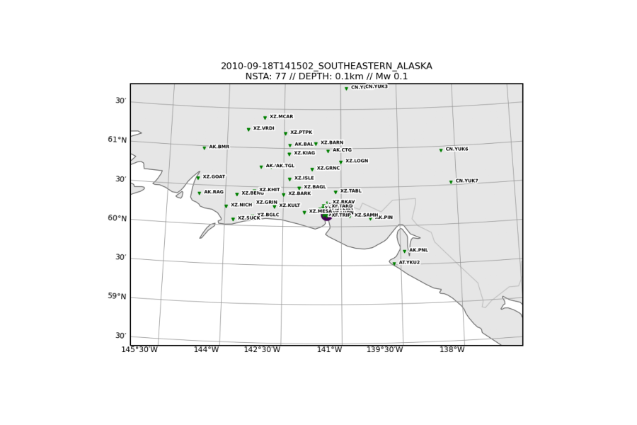
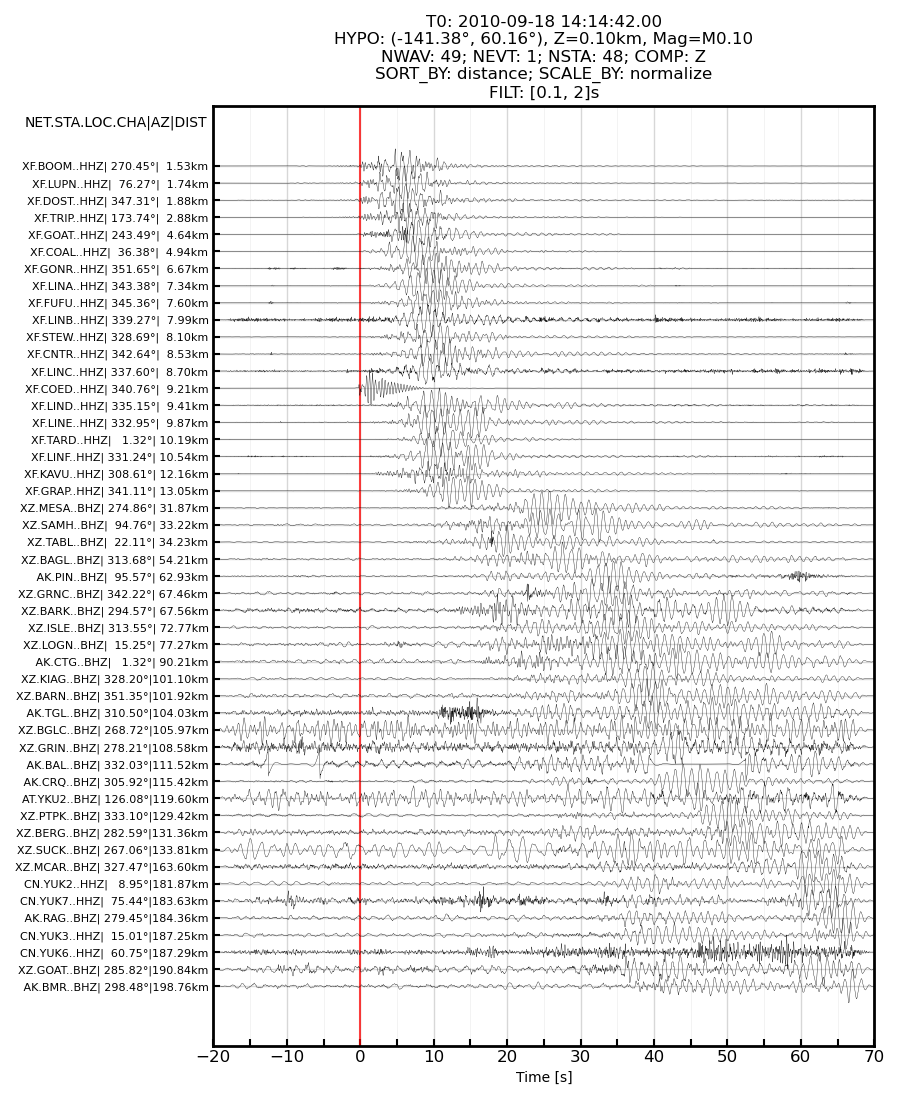
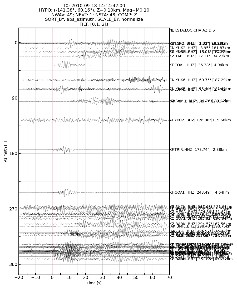
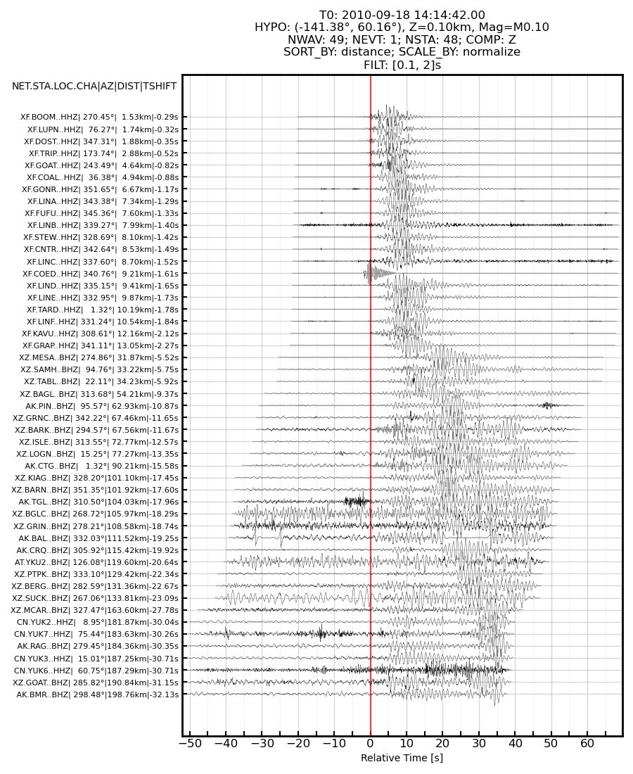
Example 1: Yahtse glacier calving event#
Exercise
Examine and then run the code cell below.
From the station map generated, examine the source–station geometry, especially closest to the epicenter.
In the record section generated, how are the seismograms ordered and aligned?
What does NET.STA.LOC.CHA|AZ|DIST represent?
What do HHZ and BHZ channels represent?
What input variables were needed to specify the bandpass?
How is a bandpass filter applied within plotw_rs()? Hint: find the online documentation.
Describe the characteristics of this signal. Do you see a distinct P wave on any seismogram? (This will be clearer later, after you have seen P waves from normal earthquakes.)
Describe some oddities within the record section.
# 1. Yahtse Glacier event
# event information could not be found on catalog

download   = copy(download_defaults)
plotting   = copy(plotting_defaults)

event      = dict( origin_time                  = UTCDateTime("2010,9,18,14,15,2"),
                   event_latitude               = 60.155496,
                   event_longitude              = -141.378343,
                   event_depth_km               = 0.1,
                   event_magnitude              = 0.1 )

duration   = dict( seconds_before_ref           = 20,
                   seconds_after_ref            = 70 )

download['channels']                            = 'HHZ,BHZ'
download['overwrite_event_tag']                 = 'Example_1'

bandpass   = dict( min_period_s                 = 0.1,
                   max_period_s                 = 2 )

plotting["pysep_path"]                          = f'{download["output_dir"]}/{download["overwrite_event_tag"]}'

fetch_and_plot(event,duration,download,plotting,bandpass)
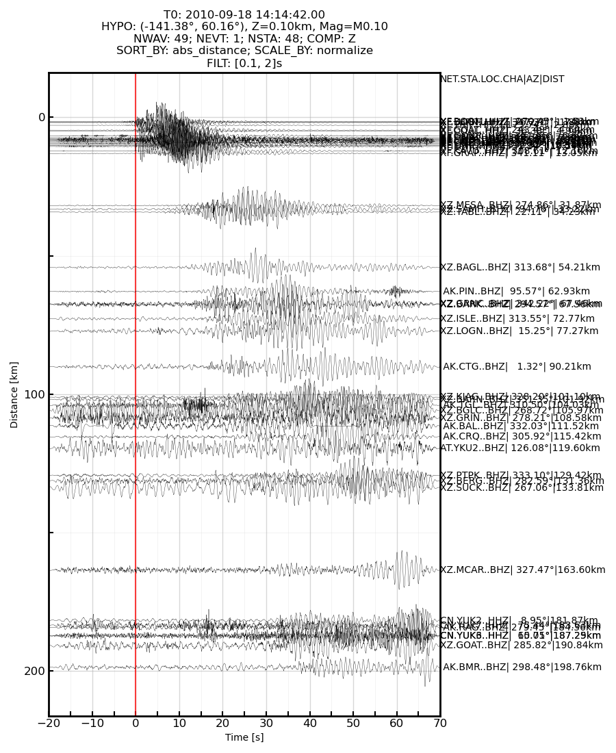
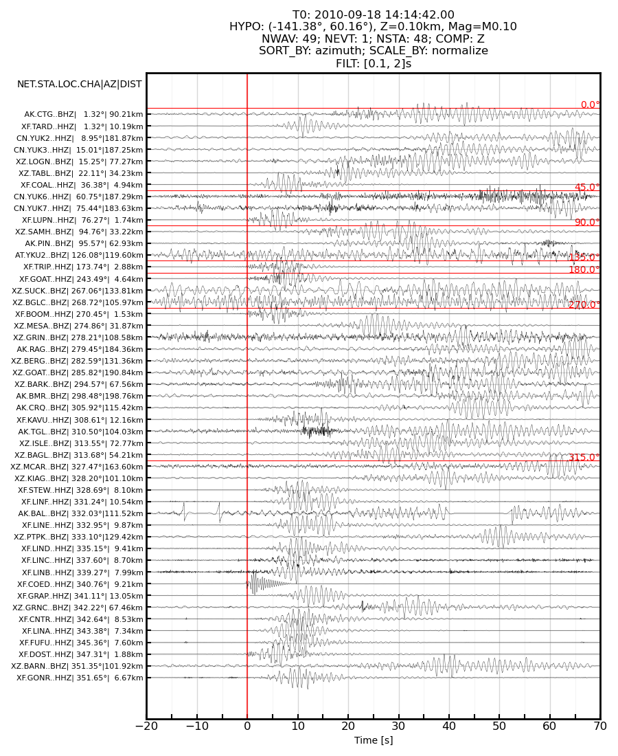
Now try out the different options for sorting seismograms in record sections by running the next cell.
You can add _r* to reverse the sorting order; for example, for alphabetical_r the sorting will go from Z to A.*
# seismogram sorting options
# set to run only for example_index = 1

sort_by_tag = ['distance', 'absolute distance', 'azimuth', 'absolute azimuth']

for i, sort_by in enumerate(['distance', 'abs_distance', 'azimuth', 'abs_azimuth']):

    print(f'\n\nCase {i+1}: Seismograms sorted by {sort_by_tag[i]}\n\n')

    plotting['sort_by']  = sort_by

    plotw_rs(**plotting, **bandpass)
Case 1: Seismograms sorted by distance

Case 2: Seismograms sorted by absolute distance
Case 3: Seismograms sorted by azimuth
Case 4: Seismograms sorted by absolute azimuth
Seismograms aligned on the S wave arrival
Now try aligning the seismograms on an arrival of your choice.
The example below aligns the seismograms on the estimated S arrival times.
# seismograms alignment on the S wave
# set to run only for example_index = 1

print(f'\n\nSeismograms aligned on the S wave arrival\n\n')

plotting['sort_by']      = 'distance'
plotting['time_shift_s'] = 's_arrival_time'

plotw_rs(**plotting, **bandpass)
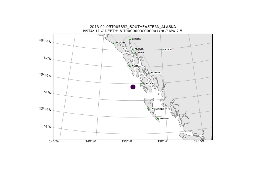
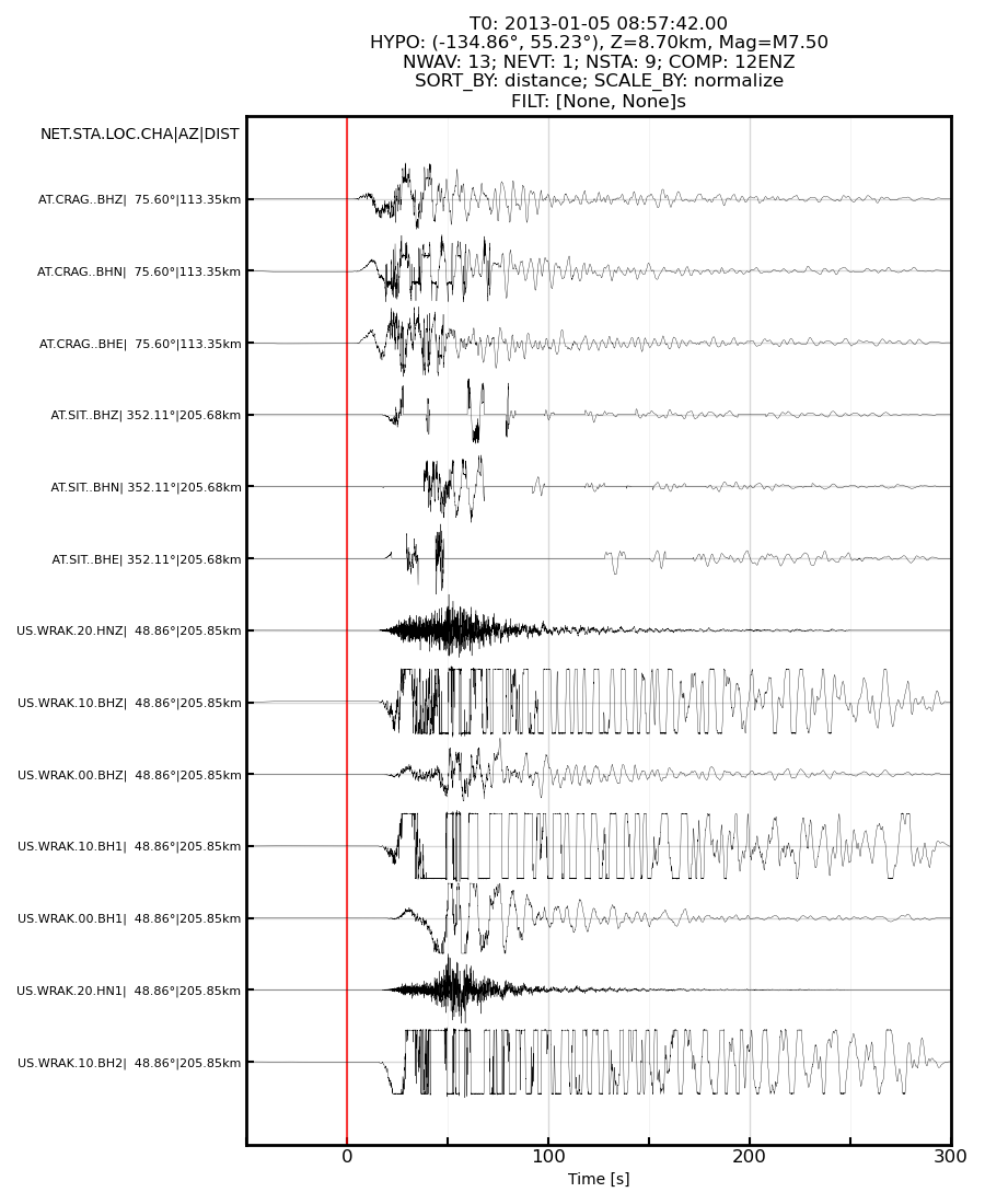
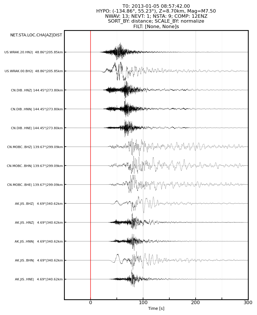
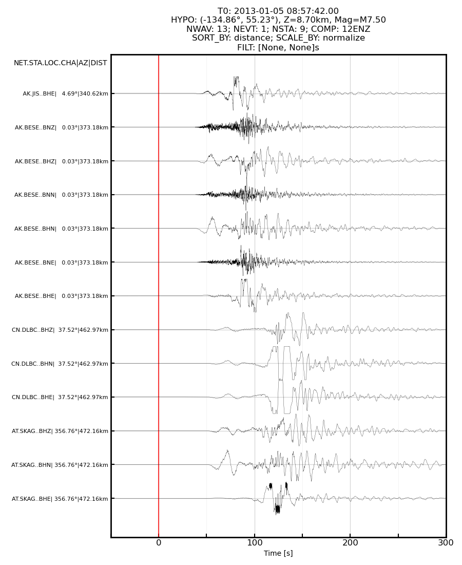
Example 2: Mw 7.5 earthquake in southeastern Alaska, near-source recordings#
Event information:
https://earthquake.usgs.gov/earthquakes/eventpage/ak0138esnzr
Exercise
Examine and then run the code cell below.
Comment on the notable features of the seismograms.
# 2. Mw 7.5 earthquake in southeastern Alaska

download   = copy(download_defaults)
plotting   = copy(plotting_defaults)

channels_1 = 'BHZ,BHE,BHN,BH1,BH2'                                           # broadband channels
channels_2 = 'BNZ,BNE,BNN,BN1,BN2,BLZ,BLE,BLN,BL1,BL2'                       # strong motion channels
channels_3 = 'HNZ,HNE,HNN,HN1,HN2,HLZ,HLE,HLN,HL1,HL2'                       # strong motion channels

# warning: waveforms will have different units (nm/s, nm/s^2)
channels   = f'{channels_1},{channels_2},{channels_3}'

event      = dict( origin_time                  = UTCDateTime("2013,1,5,8,58,32"),
                   event_latitude               = 55.228,
                   event_longitude              = -134.859,
                   event_depth_km               = 8.7,
                   event_magnitude              = 7.5 )

duration   = dict( seconds_before_ref           = 50,
                   seconds_after_ref            = 300 )

download['channels']                            = channels
download['maxdistance_km']                      = 500
download['overwrite_event_tag']                 = 'Example_2'

bandpass   = dict( min_period_s                 = None,
                   max_period_s                 = None )

plotting['amplitude_scale_factor']              = 0.5
plotting['max_traces_per_rs']                   = 13
plotting["pysep_path"]                          = f'{download["output_dir"]}/{download["overwrite_event_tag"]}'

fetch_and_plot(event,duration,download,plotting,bandpass)
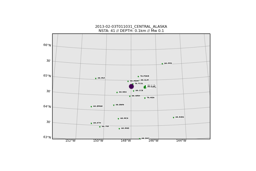
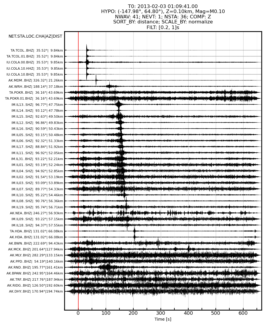
Example 3: Explosion in Fairbanks#
Exercise
Examine and then run the code cell below.
There are two signals that appear at most stations. Start by examining the station MDM (Murphy Dome).
There is only one source, so how can you explain both signals in terms of their travel times and amplitudes?
# 3. explosion in Fairbanks
# event information could not be found on catalog

download   = copy(download_defaults)
plotting   = copy(plotting_defaults)

#event location based on infrasound
#elat = 64.8156; elon = -147.9419                                            # original AEC
#elat = 64.8045; elon = -147.9653                                            # reviewed AEC

event      = dict( origin_time                  = UTCDateTime("2013,2,3,1,10,31"),
                   event_latitude               = 64.80175,
                   event_longitude              = -147.98236,
                   event_depth_km               = 0.1,
                   event_magnitude              = 0.1 )

duration   = dict( seconds_before_ref           = 50,
                   seconds_after_ref            = 200 / 0.3 )                # air wave travel time

download['channels']                            = 'SHZ,HHZ,BHZ'              # broadband channels
download['overwrite_event_tag']                 = 'Example_3'

bandpass   = dict( min_period_s                 = 0.2,
                   max_period_s                 = 1 )

plotting["pysep_path"]                          = f'{download["output_dir"]}/{download["overwrite_event_tag"]}'

fetch_and_plot(event,duration,download,plotting,bandpass)
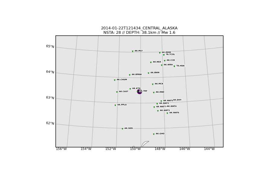
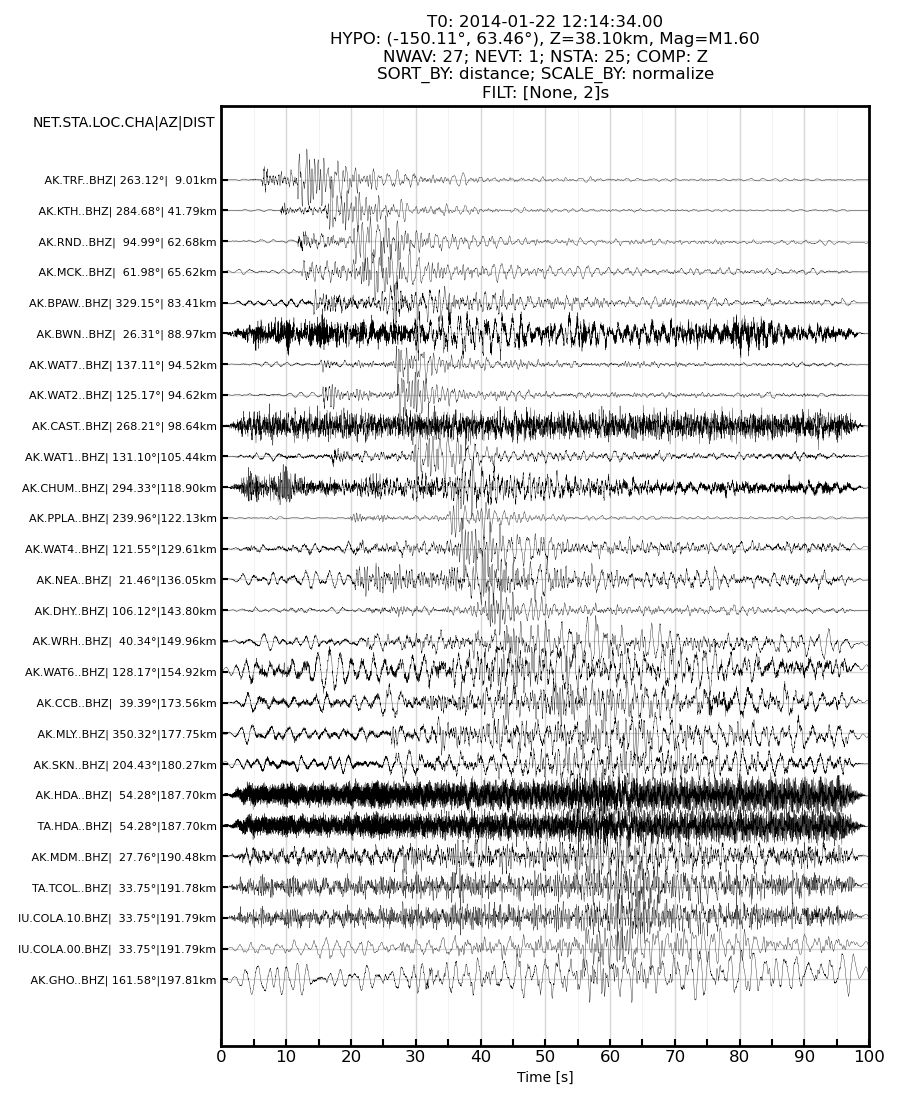
Example 4: Very low frequency earthquake near Denali#
Exercise
Examine and then run the code cell below.
Estimate the dominant frequency of this event?
# 4. very low frequency (VLF) event near Kantishna
# event information taken from IRIS

download   = copy(download_defaults)
plotting   = copy(plotting_defaults)

event      = dict( origin_time                  = UTCDateTime("2014,1,22,12,14,34"),
                   event_latitude               = 63.46,
                   event_longitude              = -150.11,
                   event_depth_km               = 38.1,
                   event_magnitude              = 1.6 )

duration   = dict( seconds_before_ref           = 0,
                   seconds_after_ref            = 100 )

download['overwrite_event_tag']                 = 'Example_4'

bandpass   = dict( min_period_s                 = None,
                   max_period_s                 = 2 )

plotting["pysep_path"]                          = f'{download["output_dir"]}/{download["overwrite_event_tag"]}'

fetch_and_plot(event,duration,download,plotting,bandpass)
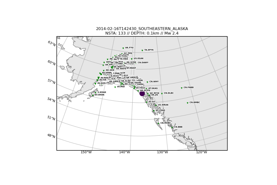
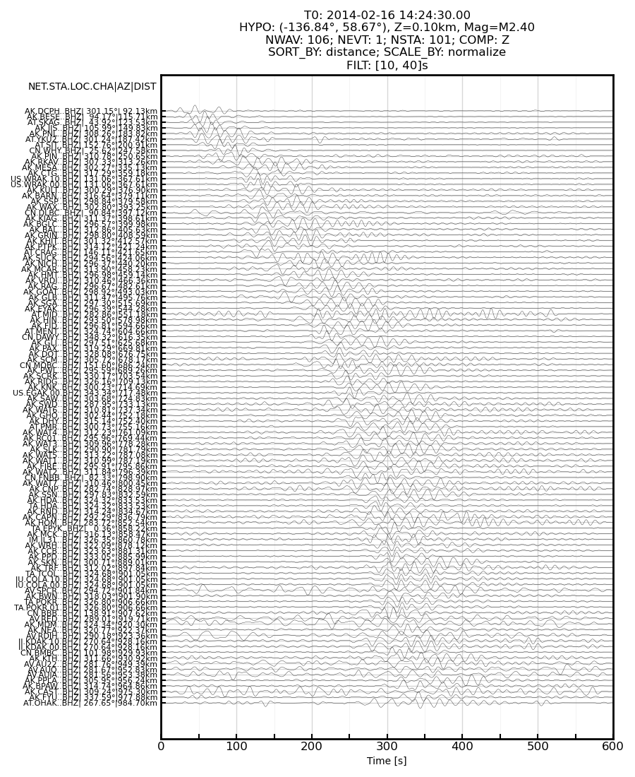
Example 5: Landslide near Lituya Bay#
Exercise
Examine and then run the code cell below.
What is the dominant frequency of this event?
# 5. landslide near Lituya Bay
# event information taken from IRIS

download   = copy(download_defaults)
plotting   = copy(plotting_defaults)

event      = dict( origin_time                  = UTCDateTime("2014,2,16,14,24,30"),
                   event_latitude               = 58.67,
                   event_longitude              = -136.84,
                   event_depth_km               = 0.1,
                   event_magnitude              = 2.4 )

duration   = dict( seconds_before_ref           = 0,
                   seconds_after_ref            = 600 )

download['maxdistance_km']                      = 1000
download['overwrite_event_tag']                 = 'Example_5'

bandpass   = dict( min_period_s                 = 10,
                   max_period_s                 = 40 )

plotting["pysep_path"]                          = f'{download["output_dir"]}/{download["overwrite_event_tag"]}'

fetch_and_plot(event,duration,download,plotting,bandpass)
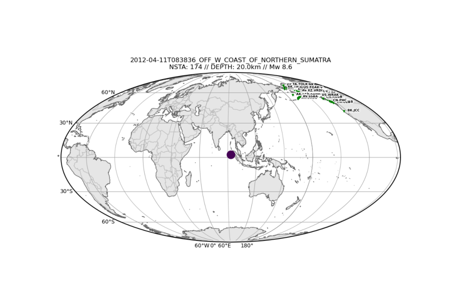
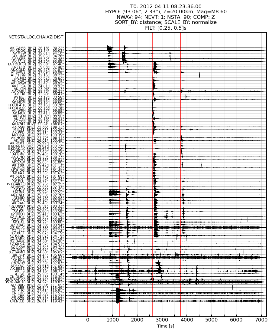
Example 6: Mw 8.6 Indian Ocean (offshore Sumatra) earthquake triggering earthquakes in Alaska#
Event information
6.1. Andreanof: https://earthquake.usgs.gov/earthquakes/eventpage/usp000jhh4
6.2. Nenana: https://earthquake.usgs.gov/earthquakes/eventpage/ak024ouaxa8
6.3. Iliamna: https://earthquake.usgs.gov/earthquakes/eventpage/ak0124ouezxl
# origin times of known earthquakes
origin_time_sumatra   = UTCDateTime("2012,4,11,8,38,36")
origin_time_andreanof = UTCDateTime("2012,4,11,9,0,9")
origin_time_nenana    = UTCDateTime("2012,4,11,9,21,57")
origin_time_iliamna   = UTCDateTime("2012,4,11,9,40,58")

# origin times, in seconds, relative to Sumatra origin time
t_andreanof = origin_time_andreanof - origin_time_sumatra
t_nenana    = origin_time_nenana    - origin_time_sumatra
t_iliamna   = origin_time_iliamna   - origin_time_sumatra
Exercise
Examine and then run the code cell below.
Examine the record section and try to determine what you see.
For each event (which we define as a signal that appears on several stations), determine what the closest station is. Where did each event occur?
Change the bandpass period range (min_period_s and max_period_s) for the record section plot to be 2–1000s, so that you see the complete frequency range of this waveform.
Approximately how long did this earthquake last in Alaska?
# 6. Mw 8.6 Indian Ocean (offshore Sumatra) earthquake

download   = copy(download_defaults)
plotting   = copy(plotting_defaults)

event      = dict( origin_time                  = origin_time_sumatra,
                   event_latitude               = 2.327,
                   event_longitude              = 93.063,
                   event_depth_km               = 20,
                   event_magnitude              = 8.6 )

duration   = dict( seconds_before_ref           = 0.25 * 60 * 60,
                   seconds_after_ref            = 2    * 60 * 60 )

stations   = dict( minlatitude                  =    64.922 - 25,
                   maxlatitude                  =    64.922 + 25,
                   minlongitude                 = - 148.946 - 25,
                   maxlongitude                 = - 148.946 + 25 )

download['maxdistance_km']                      = 6371 * np.pi
download                                        = {**download, **stations}
download['overwrite_event_tag']                 = 'Example_6'

# P wave + triggered events
bandpass   = dict( min_period_s                 = 0.25,
                   max_period_s                 = 0.5 )

# full wavetrain (no triggered events visible)
# bandpass   = dict( min_period_s                 = 2,
#                    max_period_s                 = 1000 )

plotting['distance_units']                      = 'deg'
plotting['tmarks']                              = [0, t_andreanof, t_nenana, t_iliamna]
plotting["pysep_path"]                          = f'{download["output_dir"]}/{download["overwrite_event_tag"]}'

fetch_and_plot(event,duration,download,plotting,bandpass)
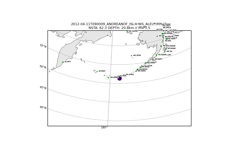
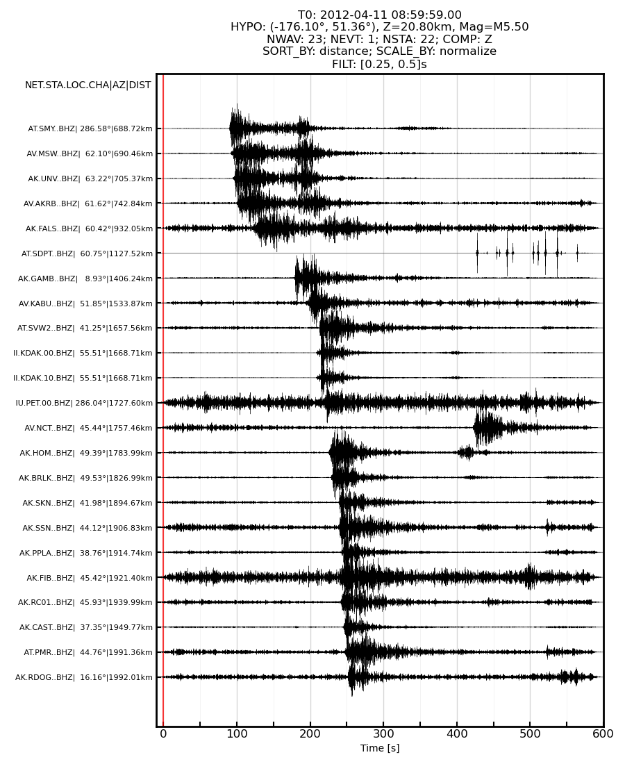
Exercise
Examine and then run the code cells for example 6.1., 6.2. and 6.3. below.
You are given the source parameters for three earthquakes that occurred in Alaska during the ground motion of the main wavetrain from the Mw 8.6 Indian Ocean (offshore Sumatra) earthquake. For each possibly triggered event, tabulate the following information:
the closest station (and the distance in km)
the suspicious stations
the widest period range over which the signal is clearly visible. This can be achieved by varying min_period_s and max_period_s provided as an input for plotting the record sections.
# 6.1. triggered earthquake - Andreanof (NEIC)

download   = copy(download_defaults)
plotting   = copy(plotting_defaults)

event      = dict( origin_time                  = origin_time_andreanof,
                   event_latitude               = 51.364,
                   event_longitude              = -176.097,
                   event_depth_km               = 20.8,
                   event_magnitude              = 5.5 )

duration   = dict( seconds_before_ref           = 10,
                   seconds_after_ref            = 600 )

download['maxdistance_km']                      = 2000
download['overwrite_event_tag']                 = 'Example_6.1'

bandpass   = dict( min_period_s                 = 0.25,
                   max_period_s                 = 0.5 )

plotting["pysep_path"]                          = f'{download["output_dir"]}/{download["overwrite_event_tag"]}'

fetch_and_plot(event,duration,download,plotting,bandpass)
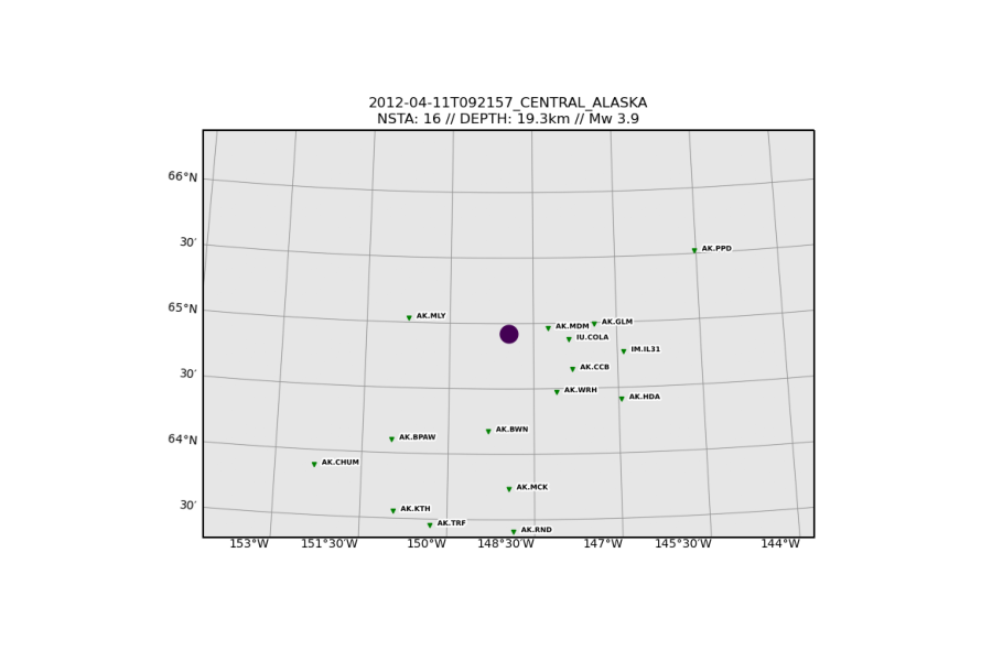
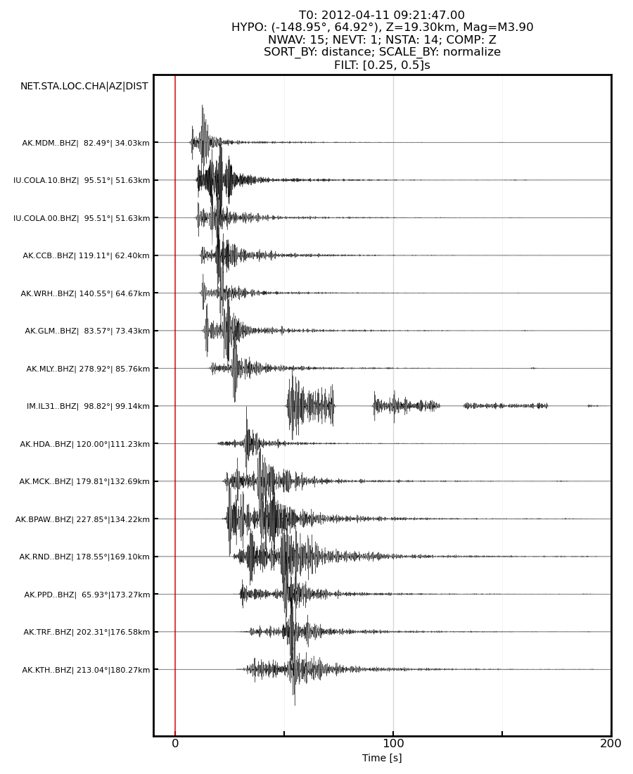
# 6.2. triggered earthquake - Nenana crustal (NEIC)

download   = copy(download_defaults)
plotting   = copy(plotting_defaults)

event      = dict( origin_time                  = origin_time_nenana,
                   event_latitude               = 64.922,
                   event_longitude              = -148.946,
                   event_depth_km               = 19.3,
                   event_magnitude              = 3.9 )

duration   = dict( seconds_before_ref           = 10,
                   seconds_after_ref            = 200 )

download['overwrite_event_tag']                 = 'Example_6.2'

bandpass   = dict( min_period_s                 = 0.25,
                   max_period_s                 = 0.5 )

plotting["pysep_path"]                          = f'{download["output_dir"]}/{download["overwrite_event_tag"]}'

fetch_and_plot(event,duration,download,plotting,bandpass)
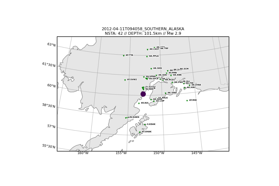
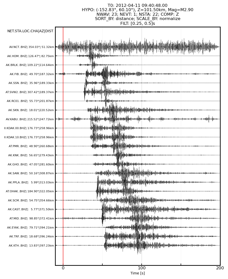
# 6.3. triggered earthquake - Iliamna intraslab (NEIC)

download   = copy(download_defaults)
plotting   = copy(plotting_defaults)

event      = dict( origin_time                  = origin_time_iliamna,
                   event_latitude               = 60.104,
                   event_longitude              = -152.832,
                   event_depth_km               = 101.5,
                   event_magnitude              = 2.9 )

duration   = dict( seconds_before_ref           = 10,
                   seconds_after_ref            = 200 )

download['maxdistance_km']                      = 400
download['overwrite_event_tag']                 = 'Example_6.3'

bandpass   = dict( min_period_s                 = 0.25,
                   max_period_s                 = 0.5 )

plotting["pysep_path"]                          = f'{download["output_dir"]}/{download["overwrite_event_tag"]}'

fetch_and_plot(event,duration,download,plotting,bandpass)
Example 7: Your own example#
Exercise
Examine and then modify the code cell below to look at an event of your interest, by extracting waveforms and plotting a record section.
# 7. your own example below

download   = copy(download_defaults)
plotting   = copy(plotting_defaults)

download['overwrite_event_tag'] = 'Example_7'
plotting["pysep_path"] = f'{download["output_dir"]}/{download["overwrite_event_tag"]}'

event      = dict()

duration   = dict()

bandpass   = dict()

# fetch_and_plot(event,duration,download,plotting,bandpass)